Background
WHO Outbreak News
Back when I worked in global infectious disease genomics, I often kept an eye on the Disease Outbreak News (DONs) from the World Health Organisation. DONs are brief reports about disease outbreaks (hence the name) and contain crucial information about symptoms, locations, and the number of individuals affected by known and novel diseases. They contain a multitude of diseases, locations and time periods.
My interest in these reports led to me to build Outbreaker, for reading these articles via the command line.
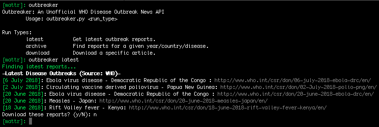
Note: The DONs website was recently restructured, breaking Outbreaker.
Latent Dirichlet Allocation
Fast forward to today and I’m working in natural language processing at Linguamatics/IQVIA. From this viewpoint, DONs are an interesting dataset to which topic modelling algorithms (essentially learning the themes found in a set of documents) can be applied. In this blog, we’ll be taking a look at Latent Dirichlet Allocation (LDA).
LDA is a generative model for learning a given number of topics in a collection of documents. This approach begins by assigning random topics to every word in every document and then iterates over those words multiple times. With each pass, the model is tweaked as the topic assigned to each word is updated according to the most probable topic for that word in that document at that time. The topics assigned to a document are therefore determined by the topics assigned to the words in that document. Even better, once we’ve built our model we can predict what topics new documents contain.
In the real world, topic modelling is useful for everything from automatically tagging news articles to identifying a subset of similar documents (such as electronic health records) for further investigation. So let’s try it out.
Data Scraping, Cleaning & Normalisation
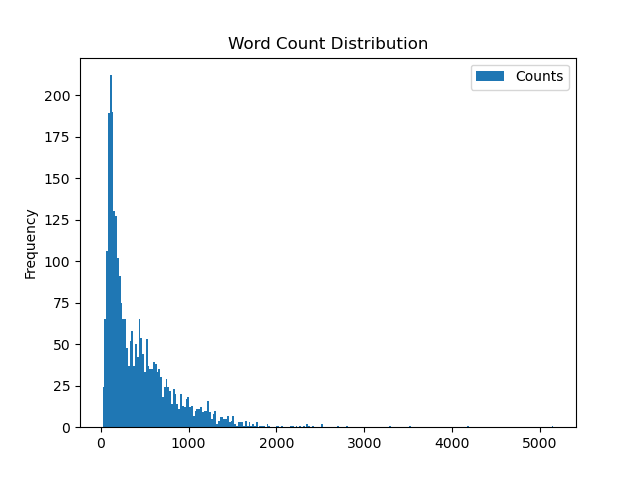
Step one is getting our dataset, here we’ll be using 2,831 reports from 1996 to 2019. Each report is relatively concise, with a mean of 428.49 words per document (σ=411.31), but there’s a long tail of longer reports. You can find the full dataset here.
Given that unstructured data is inherently messy, step two is data cleaning and normalisation.
Removing Uninformative Words
Common and generally meaningless stop words (such as and, in, and the) are often removed from training datasets to reduce noise and improve training efficiency.
In addition to the standard list provided by nltk, we’ll also be removing single characters, integers below 10, and other words found at a high frequency in our corpus (e.g. case, cases, health, report, reported, reports, and reporting). The base list can be found here.
It’s also a good idea to remove punctuation, to avoid this being seen as a different word from this!:
line = line.translate(str.maketrans('', '', string.punctuation+'—–‘’“”')).lower()
Standardising Word Variants
Variations of the same core word (e.g. cook, cooking, cooked, and cooks, all just mean cook) can be normalised through stemming, for which we will apply the Porter stemmer as implemented in nltk.
Normalising Concepts
Various concepts need to be standardised to remove superfluous details about their specific values. For example, it’s often more valuable to know that a file is present than to know what its file name is.
Therefore we will be applying the following normalisations:
| Concept Type | Normalised Word | Regex Pattern |
|---|---|---|
| Ages | <AGE> |
\d+yearold |
| Case counts | <COUNT> |
(?<!\w)n\d+ |
| File names | <FILE> |
\S*(jpg|jpeg|png|tiff|pdf|xls|xlsx|doc|docx)(?!\w) |
| Monetary values | <CURRENCY> |
(?<!\w)[$£¥€¢$﹩£¥¢₤][\d.]* |
| URLs | <URL> |
(?<!\w)http\S* |
All of these can be standardised with a regex substitute such as:
line = re.compile(regex_pattern).sub(normalised_token, line)
Countries names can also be a pain, as we don’t want multi-word names (ie. Democratic Republic of the Congo) to be split into their distinct words. To fix this, we’ll be using a lexicon of multi-word countries and replacing those multi-token names with single tokens (e.g. democratic_republic_of_the_congo), as shown below.
for multi_word_token in MULTI_WORD_TOKENS:
	multi_word_token = multi_word_token.strip()
	line = line.replace(multi_word_token, multi_word_token.replace(' ','_'))
Building the model
WIth our data (relatively) clean, it’s time to actually build our model, and whilst it’s possible to build a ‘from scratch’ method, such as described in Joel Grus’ brilliant “Data Science from Scratch”, these approaches can be incredibly slow (as Grus himself warns). Therefore, in the interests of speed & sanity I’d heavily suggest using the gensim library.
That said, you can find both the from scratch and gensim-based implementations in the associated GitHub repo. Just be warned, the ‘from scratch’ method is incredibly slow (but useful for understanding how the method actually works).
Optimising the model
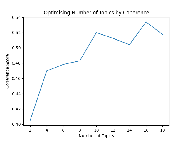
Whilst building any old model is fairly straight-forward, ultimately we want a good one. For example, we’ll want to avoid learning a purely arbitrary number of topics. One way to identify a reasonable number of topics to learn is to explore the coherence of the models we build. (We could also optimise our alpha and beta parameters, but for the sake of brevity we’ll just focus on topic coherence for today.)
Topic coherence is an approach for scoring the similarity of words within the topics we identify (well-founded and reasonable topics are more coherent). By training a variety of topic models with a range of different topic numbers, we can identify a suitable number of topics to learn.
Several metrics can be used to measure coherence, including c_a, c_npmi, c_p, c_uci, c_umass, and c_v. Each takes a slightly different approach but we’ll be using c_v coherence.
You can replicate this optimisation approach for your own models with the find_optimal_topic_number method:
modeller.find_optimal_topic_number()
This produces the following plot, from which we can propose 12 as a reasonably coherent number of topics to train for.
Actually building the model
Once we’re happy with our topic number, training the model (with the associated code), is as easy as:
modeller = Modeller("./Documents/documents_1996-2019.txt", num_topics=12)
modeller.build_model()
trained_model = modeller.export_model()
visualiser = Visualiser(trained_model)
Topic Exploration
With our model trained, we can explore some topics.
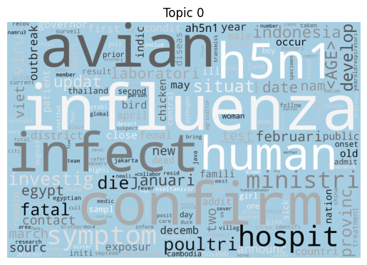
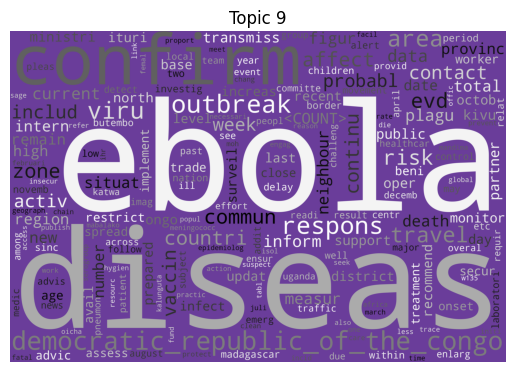
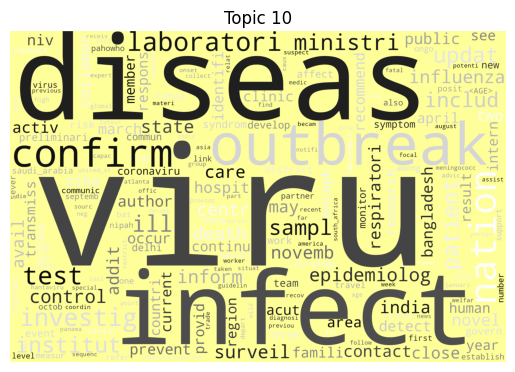
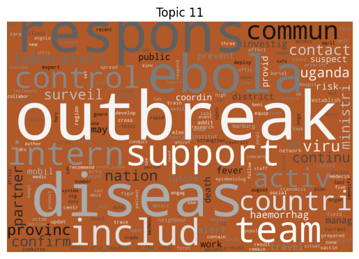
Word clouds
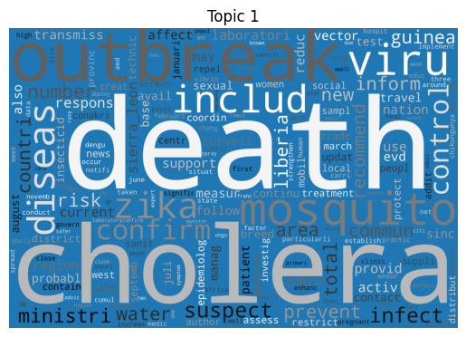
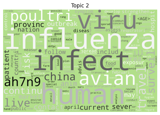
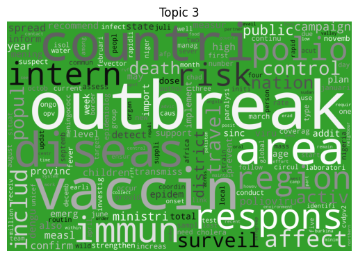
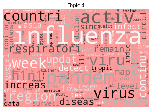
As is tradition for a bag of words output, let’s start with a word cloud for each topic (yes I know they’re awful, but they do look fancy).
To build your own, you can use the following method:
visualiser.plot_topic_clouds()
 |
 |
 |
 |
 |
 |
 |
 |
 |
 |
 |
 |
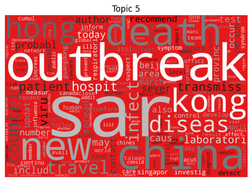
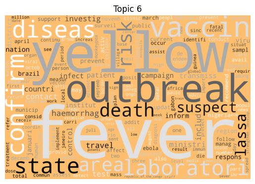
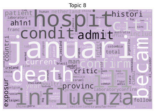
Immediately we can see some striking signals for some topics, such as ebola, diseas for topic 9 and outbreak, sar, hong, kong for topic 5. januari is also a notable token for topic 8, suggesting that this topic may be associated with a specific timeframe.
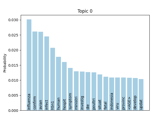
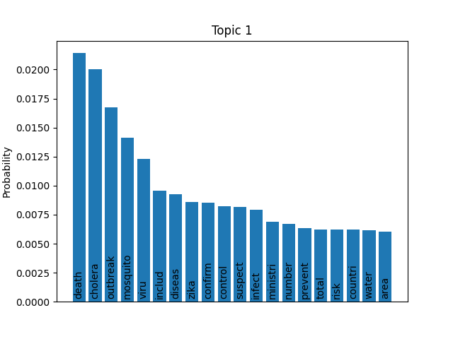
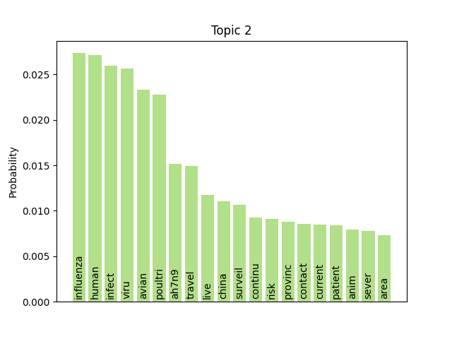
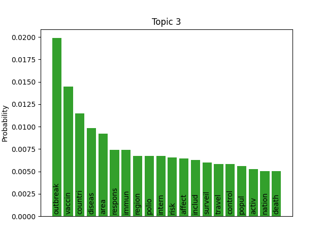
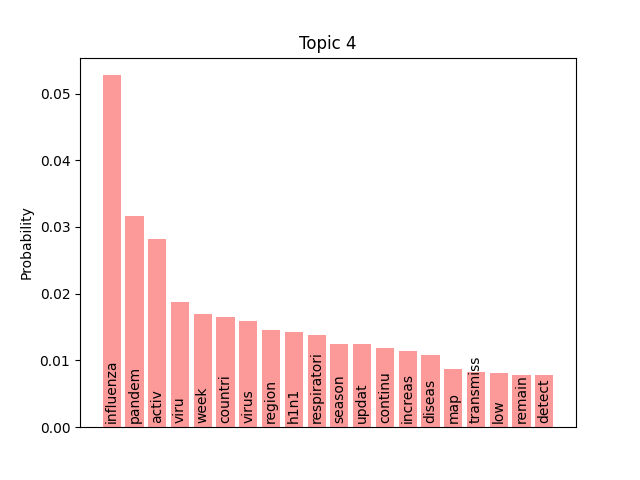
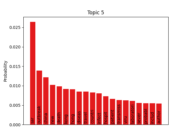
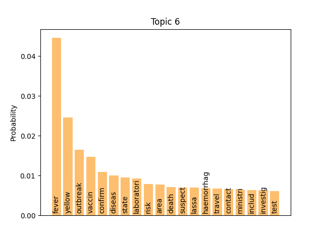
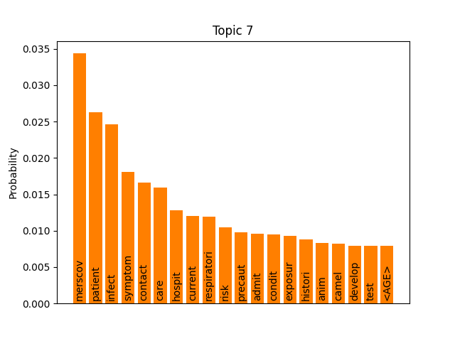
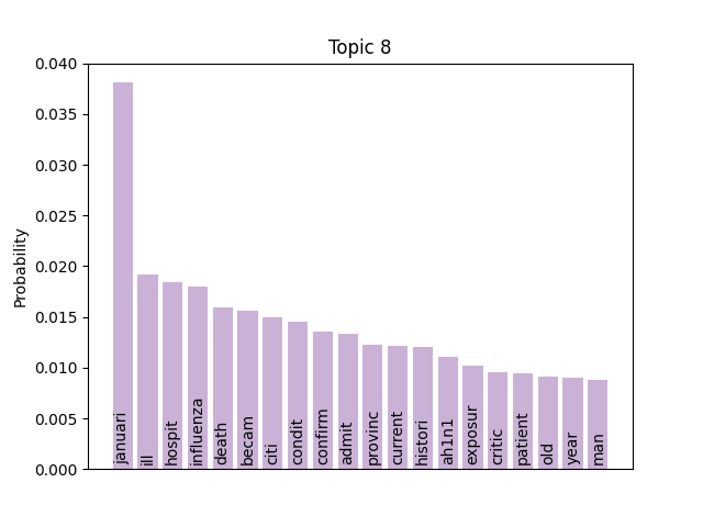
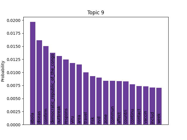
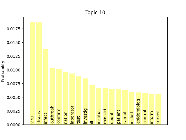
Word/topic probabilities
We can consider these notable tokens more objectively via word/topic bar charts, produced with the following method:
visualiser.plot_word_bars()
 |
 |
 |
 |
 |
 |
 |
 |
 |
 |
 |
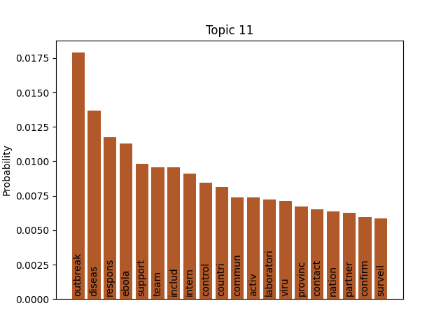 |
Here notable outliers for specific topics include spikes for influenza in topic 4, sar in topic 5, fever and yellow in topic 6, and januari in topic 8.
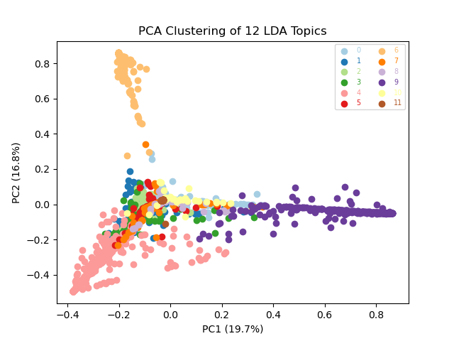
Topic-based document clustering
Dimension reduction techniques, such as PCA and t-SNE, are great for visually comparing document similarity and topic clusters. For these visualisations, our per-document topic weights are our input data. Documents with more similar topics will therefore cluster together.
visualiser.plot_pca()
visualiser.plot_tsne()
 |
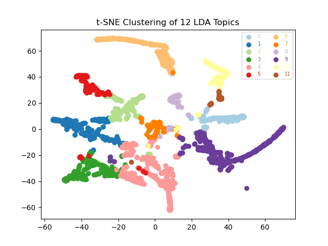 |
Broadly, our PCA shows broad overlaps between our topics, at least for the first two principle components, implying that stratification is limited (especially as Principal Component 1 only accounts for 19.7% of the total variance). In contrast the t-SNE plot suggests that topics 6 and 9 are relative outliers, and that a small subset of documents are clustering amongst other topics.
Our documents generally cluster together according to their topics but our topic clusters are not dramatically distinct from one another (an exception to this is topic 6). This is probably to be expected as our documents are all disease outbreak reports, and so their content is not going to vary dramatically. Beyond the specific diseases and locations of interest, a lot of the text is probably going to appear fairly similar.
Time-based clustering
Given that the documents are ordered in time, we can explore the change in topic distribution over document order with the following method:
visualiser.plot_doc_topics()
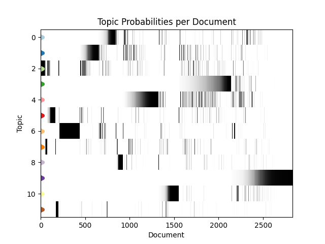
This shows us that our topics are grouped into time-based clusters, which makes a lot of sense. When disease outbreaks occur, we’re going to get a stream of reports one after the another in a fixed timeframe as the outbreak progresses.
Another interesting phenomena here is that topic probabilities appear to be ‘fading in’ over time, with documents earlier in an outbreak being less strongly associated with that topic. This most probably reflects the fact that early disease reports are going to contain less distinctive, more vague information about that outbreak. For example, fewer symptoms or locations may be known and the disease or strain may not been named or identified yet.
With this information we can further elucidate our topics, for example topic 9 features a very recent (end of 2019) cluster of reports that mention Ebola - making these likely referring to the 2018–2020 Kivu Ebola epidemic. Further back in time, we see a cluster of topic 0 documents that appear to be linked to the spread of H5N1 in 2004.
Quintessential documents
One final strategy for characterising our topics is to manually examine the highest probability documents for each topic, as these effective represent the best example of a document for its associated topic. You can extract these documents from your model with:
modeller.find_representative_documents()
For us, those documents are:
| Topic | Example Document | n. Docs (P≥0.95) |
|---|---|---|
| 0 | Avian influenza A(H5N1) - update 14 (…) | 238 |
| 1 | Zika virus infection – Saint Lucia | 49 |
| 2 | Human infection with avian influenza A(H7N9) virus – China | 102 |
| 3 | Circulating vaccine-derived poliovirus type 2 – African Region | 111 |
| 4 | Pandemic (H1N1) 2009 - update 94 | 56 |
| 5 | Update 62 - More than 8000 cases reported globally (…) | 56 |
| 6 | Yellow fever – Brazil | 65 |
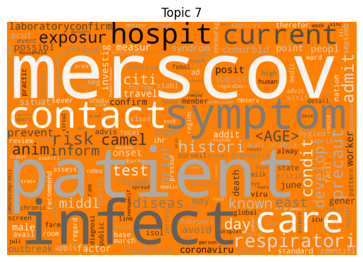
| 7 | Middle East respiratory syndrome coronavirus (MERS-CoV) – Saudi Arabia | 240 |
| 8 | Human infection with avian influenza A(H7N9) virus – update | 29 |
| 9 | Ebola virus disease – Democratic Republic of the Congo | 58 |
| 10 | Influenza & Nipah virus - India | 16 |
| 11 | Ebola haemorrhagic fever in the Democratic Republic of the Congo - update 2 | 52 |
A note on pyLDAvis
Quick side note to mention that I also explored pyLDAvis for LDA visualisations, but encountered a few issues:
- Output stylesheets were missing, which broke several things.
- The standard output is an HTML file, which isn’t great for including in this blog.
That said, if you’re keen on getting pyLDAvis visualisations, you can use the visualiser.plot_pyldavis() method to generate them.
Topic Summary
Now that we’ve had a chance to investigate our topics from various angles, we can pin down our topic names. In this case, I’ve settled on the following:
| Number | Name | n. Docs (P>0.5) |
|---|---|---|
| 0 | H5N1 Influenza | 422 |
| 1 | Zika, Guillain-Barré, Chikungunya, Dengue, West African Ebola | 214 |
| 2 | A/H7N9 Avian Influenza (& other bird flus?) | 152 |
| 3 | Poliovirus (inc. vaccine references) | 405 |
| 4 | H1N1 Swine Flu Pandemic | 70 |
| 5 | SARS-CoV, esp. 2002-2004 outbreak | 156 |
| 6 | Yellow Fever | 270 |
| 7 | MERS-CoV | 307 |
| 8 | H1N1 Influenza Lab Confirmations | 54 |
| 9 | Ebola, esp. the 2018–2020 Kivu Ebola epidemic | 121 |
| 10 | Nipah virus, Central American Zika, ARS | 85 |
| 11 | Ebola, especially its control | 199 |
Predicting Topics in New Documents
With our model build and our topics interpreted, we can classify new documents into those topics. For example, let’s say it’s January 2020 and you’ve just finished reading a report on a pneumonia of unknown cause (spoilers, we’re talking about the initial COVID-19 disease outbreak report from 5 January 2020) - which topic (or topics) does that report most likely contain?
For this, we’ll pass our new document to the predict_topic method :
visualiser.predict_topic('./Documents/pneumonia_of_unknown_cause.txt')
Which returns:
Modeller - INFO - Predicting topic for given document
Modeller - INFO - Parsing input document: ./Documents/pneumonia_of_unknown_cause.txt
[(2, 0.60327667), (3, 0.106589556), (5, 0.25196746), (7, 0.03303717)]
Our topic prediction tells us that the new report does not fit nicely into a single topic but instead represents a combination of four: A/H7N9 Avian influenza (2), SARS-CoV-1 (5), Poliovirus (3), and MERS-CoV (7). This aligns with both the information available at the time and with what we’ve learnt since. For example, we now know that SARS-CoV-2 is closely related to SARS-CoV-1 and MERS-CoV, but was also able to spread widely and rapidly with similar symptoms to influenza pandemics.
| Topic ID | Probability | Topic Name |
|---|---|---|
| 2 | 0.692 | A/H7N9 Avian influenza |
| 5 | 0.173 | SARS-CoV-1 |
| 3 | 0.092 | Poliovirus |
| 7 | 0.039 | MERS-CoV |
In Conclusion
LDA is an awesome unsupervised machine learning method for both learning the topics present in a set of documents and for automating the classification of new documents into those topics. If I were to continue exploring this dataset further improvements could be found by identifying the optimal alpha and beta parameters for the model and investigating larger numbers of topics. I hope that I’ve demonstrated some powerful clustering and visualisation approaches that you can use to validate, digest, and communicate your own findings.
You can find all the code used in this analysis on GitHub.