I’ve recently been learning how to build simple neural networks in an attempt to nail the basics. This post is my attempt at summarising what I’ve learnt and sharing that information with others. A range of resources were used for this mini-project, but I’d like to give a specific hat-tip to a brilliant two-part blog by @iamtrask.

What is a Neural Network?
As the name implies, neural networks are biologically inspired mathematical models that adopt the interconnected behaviour of neurons.

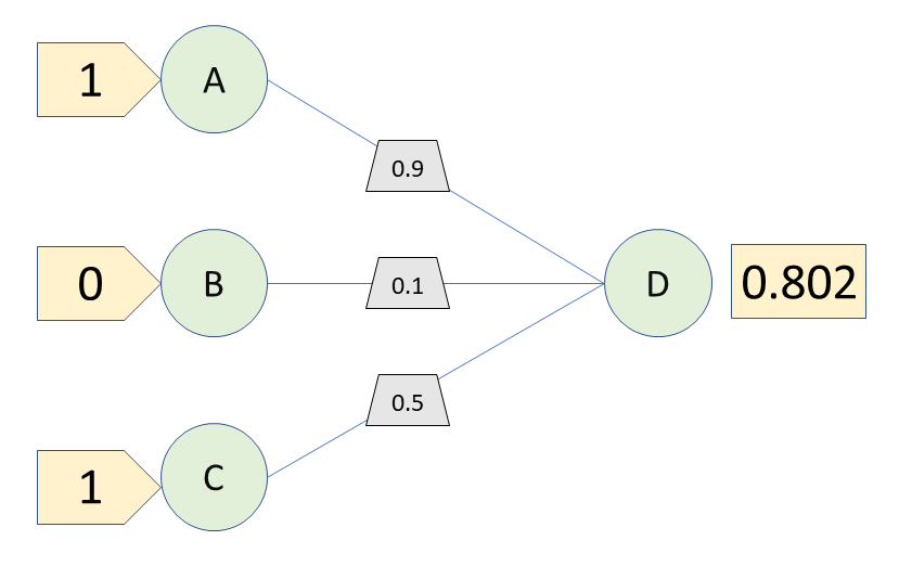
A very simple neural network might consist of three input neurons (A, B and C) outputting a signal to a third (D). Depending on whether a neuron A, B and C fire, D may also fire. But not all neuron to neuron connections are the same. For example, neuron A’s signal may be particularly informative and weighted 0.9, neuron B’s signal may be barely informative and weighted 0.1, whilst C may be averagely informative and weighted 0.5. Input to D therefore becomes the sigmoid function (see below) of (A’s state * 0.9) + (B’s state * 0.1) + (C’s state * 0.5), where the input neuron’s state is either 0 (off) or 1 (on). So let’s say that A is on (1), B is off (0) and C is on (1). The probability that D is on becomes the sigmoid function of (1*0.9) + (0*0.1) + 1*0.5). ie. 0.802, or 80.2%.

The power behind this method is that the status of a neuron can correspond to any specific factor, perhaps A is whether or not an animal has whiskers, B is whether or not an animal has fur, and C’s status is whether or not an animal has four legs. D could therefore indicate whether or not that animal is a cat.

Naturally, this is a simplification but the gist is there. Plus, it can all go a bit crazy when we start increasing the size of the neural network with more neurons and layers. In short, additional layers between the input and output layers (so called ‘hidden’ layers) will encode combinations of input neurons.

Now that’s all well and good, but how do we know which weights to apply to which connections? Simple, we iterate through the model n thousand times with a set of training data, each time shifting our neuron-neuron weights so that the model’s output is closer to the expected outputs. These weights can then be used to classify new datasets.

Pipeline In Summary
We can code this core functionality as follows:

• Begin with a training set of inputs ([1,0,0], [1,0,1], etc.) and their known outputs ([0],[1], etc.).
• Assign initial (and at first random) weights to all neuron-neuron connections. Make this a matrix of dimensions (number of neurons in layer n) * (number of neurons in layer n+1).
• Run the training dataset through the network and compare the output to the known truth.
• Calculate the distance from our network’s output to the expected output (ie. the error).
• Feed this error (times our confidence regarding the output, more on this later) back into the weights to nudge them towards accuracy.
• Repeat this weight correction for, say, 10,000 iterations.
• Use our (as accurate as they can be for now) weights on new test datasets for categorisation.

Example Script
Most tutorials exploring basic neural networks will feature a script or two for the creation of specific sizes of neural networks (I’ve recreated a couple of them on my github. I’ve also created a base class for the creation of neural networks of any size (ie. any number of layers and neurons). You can also find that script on my github.

To run the code simply:

1. Import the NeuralNetwork module.
2. Create an instance of the NeuralNetwork class, specifying size, number of eons, seed etc.
3. Train the model, either on the included training dataset or your own inputs.
4. Test the model, giving a test dataset input (the learned weights are automatically stored after training, but can also be returned).

import NeuralNetwork as NN
n = NN.NeuralNetwork(size=[3,1], eons=10000)
n.train(trainingInputs=np.array([[0,0,1],[0,1,1],[1,0,1],[1,1,1]]), trainingOutput=np.array([[0,0,1,1]]).T))
n.test([1,0,0])
0.9999370428352157

Here our output is 0.9999, suggesting very high confidence for an input of [1,0,0] corresponding to the 1 classification.

Opportunities For Expansion
We’ve only touched on the bare minimums of neural networks, so here are a couple features which we could also include:

• Drop-out: As with any other machine learning technique, neural networks can suffer from overfitting (high accuracy on training data, but low accuracy for test data). To counter this, random neurons could be removed (dropped out).
• Softmax: For networks with multiple outputs, a softmax layer after the output layer will ensure that all outputs sum to 1.0. This allows our final values to be interpreted as probabilities, and is particularly useful if utilising the ReLu activation function (rather than the sigmoid function used here).
• More complex interaction structures and neuron types (ie. memory gates etc.). Here’s a quick glimpse.

Key Elements To Consider

Sigmoid function

Given an input value, (ie. the product of signals into a node/neuron and their weights), normalise to a 0 to 1 scale. Where 0 is no firing, and 1 is firing. You can also think of it as the probability of a neuron firing. Crucially, the sigmoid function is not the only option here (others include the hyperbolic tangent and rectified linear unit (ReLu) but I’ll save those for later).

Sigmoid derivation

Given the output of a sigmoid conversion, find the gradient at that position. This is used to weight the trained weights such that neuron outputs close to 0 or 1 (ie. those with more confidence) experience smaller corrections than those with less certainty (ie. 0.5). This is an example of gradient descent.